Instructions for developing new pages for the MarineOmics webpage
Initial publication year: 2022
How to cite
Overview
If you are interested in submitting new content to the MarineOmics.github.io website, this is the guide for you! While the website managers will work with you to help prepare and publish your new page, this guide can be a useful resource as you develop your content. Below we provide general instructions as well as examples of how to build specific features (eg., tables, code chunks). Prior to developing new pages, please first contact the current Website Manager Jason Johns (jasonjohns[at]ucsb.edu). Do not hesitate to reach out with any other questions, comments, or features you’d like added to this guide.
The MarineOmics website is published through Github Pages directly from the MarineOmics github repository. In short, each page of the website is rendered as an .html from an RMarkdown (.Rmd) document. The two most important files for publishing the general website are the _site.yml and the index.Rmd/index.html.
**_site.yml**: the ‘under the hood’ backbone of the website, where things like the visual appearance of the website and the navigation bar are specified
index.html: rendered from index.Rmd - the home page from which all other pages branch
* The website manager will modify the index.html and .site_yml files for your page when you are ready to publish it, so you don’t need to know exactly how they work, but it’s good to know what they are at a basic level.
MarineOmics publishing process
Content development and review process
- Initiation: The potential contributor contacts the website manager
via email (jasonjohns[at]ucsb.edu) or the discussion forum with an idea.
- Development: Meet with the website manager, Katherine Silliman
and/or Sam Bogan (Working Group Co-leaders).
- All active members will be invited to be involved in the review
process.
- The contributor presents their idea for new material to any involved
working group members.
- There will be regular meetings (frequency decided by those involved)
with the website manager, Katherine Silliman and/or Sam Bogan, and any
other participating members for progress updates and support.
- All active members will be invited to be involved in the review
process.
- Review: Full drafts of content will be reviewed by the website manager, Katherine Silliman and/or Sam Bogan, and at least one other active MarineOmics member assigned to the project.
- Publishing: Final versions of content will be published with the help of the website manager. Please have a list of all software dependencies necessary for your .Rmd to be rendered so we can add it to our MarineOmics conda environment.
*See the bottom of the page for our policy on disagreements or conflicts during the development process
Please include the initial publication date (year at minimum) at the top of your page so it can be properly cited. We also ask that you include the below text at the top of your page, which will make a link to a section on the main website about how to cite.
[How to cite](https://marineomics.github.io/#How_to_Cite)R Markdown basics
The rendered .Rmd and .html files for each page on this site can be seen in the MarineOmics github repository. It is possible to use .Rmd files in base R, but we recommend using RStudio. If you don’t have much experience with RStudio, it’s quite intuitive with a shallow learning curve and many existing online resources for using it. It is possible to use .Rmd files in base R, but we recommend using RStudio.
Note: it’s a good idea to look at existing .Rmd scripts (including the one that codes for this page) to see examples of how a particular feature can be accomplished, such as citing references, linking a website, building a table, incorporating figures, etc. We will explicitly go over some of those features below, but there are many other bells and whistles that can be explored through online resources.
Here are some general RMarkdown tutorials that we like to reference:
- Chapter
10 from RMarkdown the Definitive Guide: Xi, Allaire, & Grolemund
2022
- R
Markdown Websites: Garrett Grolemund
Formatting basics
One of the strengths of .Rmd documents is their versatility. They can hold everything from code (not only in R but in other languages), formatted text, figure outputs, and more. Basically, code must be enclosed within ‘code chunks’ and anything outside of code chunks will be read as text, similar to a basic text file.
code chunks
Below is a basic R code chunk which can be inserted by clicking the
green +C button on the RStudio toolbar or typing the keyboard shortcut:
- macOS: command + option + I
- Windows/Linux: control + alt + I
```{r, echo = TRUE, include = TRUE}

#Here's a simple linear model in R as an example
my_lm <- lm(y ~ x, data = df)

```
Whether code chunks and/or their output are included in the knitted
.html can be modified with the logical commands “echo” and “include”.
- echo: include the code chunk itself or not
- include: include the output of the code chunk or not
* Other options exist for code chunk output which can be explored online and in other .Rmd scripts in this repository.
global code chunk options
This is the chunk where we establish global settings for the entire document. This is done with the command from the knitr package “opts_chunk$set” as shown in the example below. This command is typically included in the first code chunk, where we also load our page formatting packages and adjust the settings for citations. When a new .Rmd is made, this command is automatically included in the first chunk, which is named “setup” by default. The name of a code chunk can be specified after the r in ```{r ____}.
```{r setup}
knitr::opts_chunk$set(echo = FALSE, message = FALSE, warning = FALSE, cache = TRUE)
# load page formatting packages
library(knitr)
library(knitcitations)
library(kableExtra)
knitr::opts_chunk$set(fig.width = 10, fig.height = 5) #setting the dimensions for figure outputs in a different line of code for cleanliness
cite_options(citation_format = "pandoc", max.names = 3, style = "html",
             hyperlink = "to.doc") #setting format for in-text citations for the references section at the bottom of the page
```
* Note the “cache =” option. When set to “true” R will cache all of the output created from knitting the RMarkdown document. This is especially useful for pages with heavy computation that take a long time to knit.
including code from another language
In addition to R code, we can also run code such as bash shell script
in the R markdown file by modifying the code chunk header as below:
```{bash, eval = T}

# Here's a simple line of bash as an example
echo "Hi world"

```
formatting text
Options abound for formatting text in .Rmd documents using Pandoc Markdown, and many of
these can be found with a quick search, but we will go over a few basics
here.
- As with writing code, any text symbol that codes for something, such
as a # or a * must be escaped with a backslash (\) if you just want to
use the symbol itself.
- #: Outside of a code chunk, pound signs
dictate the size and organizational level of the text. A single # will
make large text and a main section in the navigation window. Two ## will
make slightly smaller text and a sub-section in the navigation window.
- For example, the “RMarkdown formatting” text and category was
created with “# RMarkdown formatting” while the “code chunks”
subcategory was created with “## code chunks.”
- For example, the “RMarkdown formatting” text and category was
created with “# RMarkdown formatting” while the “code chunks”
subcategory was created with “## code chunks.”
- *: Asterisks are used to bold and italicize when
surrounding texts. Use **two asterisks to bold** and
*one asterisk* to italicize.
- <br>: adds a line break
- <hr />: adds a horizontal line across the page
in-text citations from your .bib
In-text citations can be made throughout the document that will
automatically add a reference to your reference section via the
following steps:
- add your citations to the common-bib_01.bib document by exporting BibTeX-formatted citations from your reference manager
- add the line ‘bibliography: common-bib_01.bib’ to your header at the top of the .Rmd document, which looks like this:
---
title: "Instructions for developing new pages for the MarineOmics webpage"
bibliography: common-bib_01.bib
---- include the ‘cite-options’ chunk in your ‘setup’ code chunk. See the initial ‘r setup’ chunk above for the syntax of the ‘cite_options’ command.
After following these steps, you can cite them in the RMarkdown
document. Let’s say you have a paper you want to cite by LastName et
al. 2023 and the paper’s ID in your .bib file is ‘LastName2023-xy’. We
can reference this paper in-text by adding [@LastName2023-xy] to the end
of a sentence. This will produce a reference such as the one below for
Tripp et al. 2017.
syntax in .Rmd text (not in a
code chunk):
RADseq can produce insightful analyses even in the absence of data, if missing values are handled properly [@Tripp2017-cp].knitted output:
RADseq can produce insightful analyses
even in the absence of data, if missing values are handled properly
(Tripp et al. 2017).
You can also add hyperlinks to each in text citation that direct to
the References section at the bottom of the page. The in text citation
keeps its normal format, but with brackets added around the parentheses.
Directly after the citation (also in parentheses) is the ‘#’ link to the
References section: (#refs) in this case.
.Rmd: [(@Tripp2017-cp)](#refs)
rendered
html: (Tripp et al.
(2017))
At the bottom of the .Rmd, where the ‘##
References’ heading is, we have a ‘{#refs}’, which creates the target
for all links with ‘(#refs)’. It looks like this on the .Rmd:
##
References {#refs}
installing & loading packages
If you will be using any R packages or external software for your
content, it’s a good idea to highlight them toward the beginning of your
page, including code for installing them. Here’s an example from the
RADseq tutorial:
If you would like to run the R code
examples that are scattered throughout the guide (recommended but not
required!), you will need to install some R packages. Only need to run
this code once:
install.packages("tidyverse")
if (!requireNamespace("BiocManager", quietly = TRUE))
    install.packages("BiocManager")
#the BiocManager package facilitates the installation of packages from the Bioconductor project
BiocManager::install("SeqArray")
BiocManager::install("SNPRelate")
These external software are referenced in the tutorial:
caching
If your page includes any code that takes a long time to run, please set “cache = TRUE” in the knitr::opts_chunk$set command in your global code chunk.
Examples of how to include visual feautures such as tables, images, equations, etc.
insert a table
text in .Rmd (not in a code chunk):
| Term A | Term B | Term C | Term D | Term E | Term F | Term G |
| :--- | :--- | :--- | :--- | :--- | :--- | :--- |
| xxx | xxx | xxx | xxx | xxx | xxx | xxx |
| yyy | yyy | yyy | yyy | yyy | yyy | yyy |
| zzz | zzz | zzz | zzz | zzz | zzz | zzz |
knitted output:
| Term A | Term B | Term C | Term D | Term E | Term F | Term G |
|---|---|---|---|---|---|---|
| xxx | xxx | xxx | xxx | xxx | xxx | xxx |
| yyy | yyy | yyy | yyy | yyy | yyy | yyy |
| zzz | zzz | zzz | zzz | zzz | zzz | zzz |
You can generate a Markdown-formatted table using a free online editor, such as this one. The kableExtra package has a lot of functionality for fancier tables.
insert an image
To insert an image, you need the image file to also be uploaded to the Github repository. We store the images hosted on the website in each page’s folder and call them accordingly. For any image, please make sure you have permission to share the image and that it is appropriately cited.
code chunk in .Rmd:
```{r, echo = TRUE, include = TRUE, out.height = "40%", fig.align = "center", fig.cap="Figure from Rivera et al. 2021"}

knitr::include_graphics("ADMIN_01_submissions_instructions_files/Rivera_etal_fig.png")

```
knitted output:
knitr::include_graphics("ADMIN_01_submissions_instructions_files/Rivera_etal_fig.png")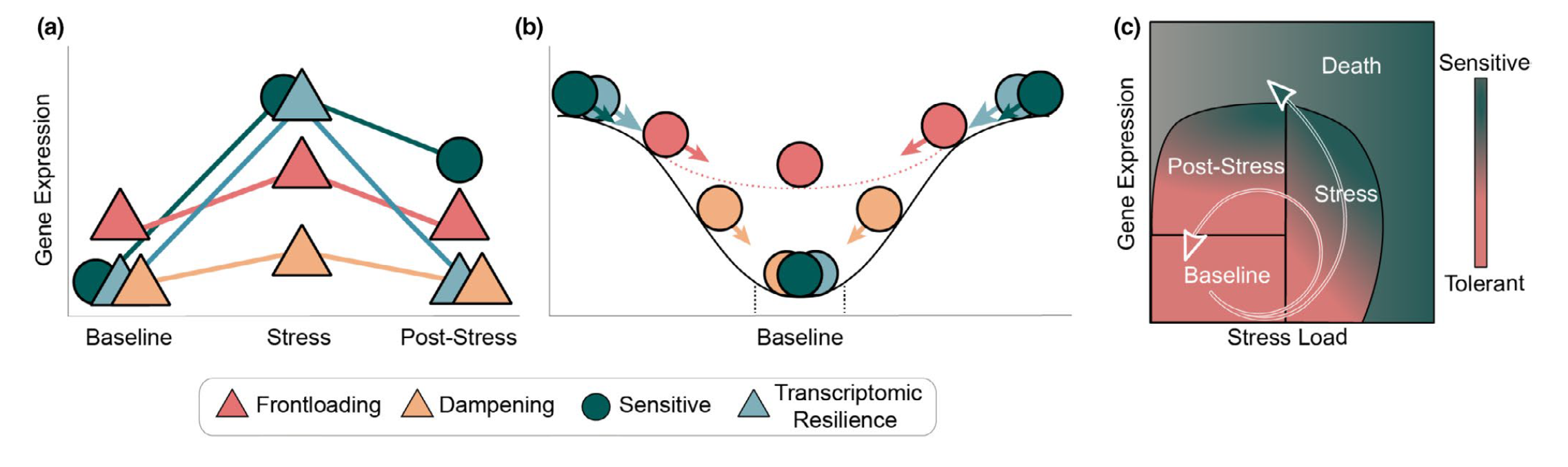
Figure from Rivera et al. 2021
write and print an equation
Equations follow LaTeX style formatting.
For illustrative purposes, here is a simple and famous equation.
syntax in .Rmd:
$$
E = mc^2
$$
knitted output: \[
E = mc^2
\]
As an example of a more complex equation, here is an equation for the
t-statistic:
syntax in .Rmd:
$$
t = \frac{\overline{x_{1}}-\overline{x_{2}}}
{\sqrt{(s^2(
\frac{1}{n_{1}} + \frac{1}{n_{2}}
))}}
$$
knitted output: \[ t = \frac{\overline{x_{1}}-\overline{x_{2}}} {\sqrt{(s^2( \frac{1}{n_{1}} + \frac{1}{n_{2}} ))}} \]
After you have finished editing your R markdown file, you can “knit” it to an HTML file by selecting the Knit button at the top of RStudio. You can review this HTML file to get an idea of what the page will look like on the website (minus the navigation bar and other site-specific formatting). You will need to upload both the R markdown file and the HTML file to Github prior to you page being added to the website.
Content/wording conflicts
At any point in the process, disagreements on what content to include
may arise. These include but are not limited to: recommendations for
experimental design, techniques, and phrasing. All disagreements will be
approached with the same method(s).
Disagreements will be
discussed with all of those involved at the time that the disagreement
arises. The first attempt at resolving the disagreement will be via
discussion. If a resolution is not agreed upon by all parties through
discussion, it will be put to a majority vote including all of those
actively involved at the time, not including the content author. In case
of a tie, a MarineOmics senior scientist will be assigned to break the
tie.